Methods
In our lab we combine computational and experimental methods in order to get the best possible understanding of our research. Our 'wet lab' enables us to measure our own data and test theoretically derived hypotheses.
MODELING METHODS
-
Ordinary differential equations
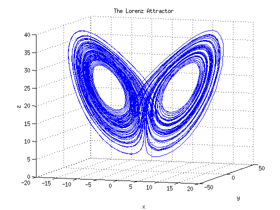
The use of ordinary differential equations (ODEs) is the most common approach to dynamic modeling. ODE modeling allows the deterministic and continuous simulation of a biological system. As such, ODEs describe the change of something in dependence to a certain variable, mostly time. ODEs are used, for example, to describe concentration changes of cellular entities, such as metabolites, mRNAs, and proteins. -
Partial differential equations
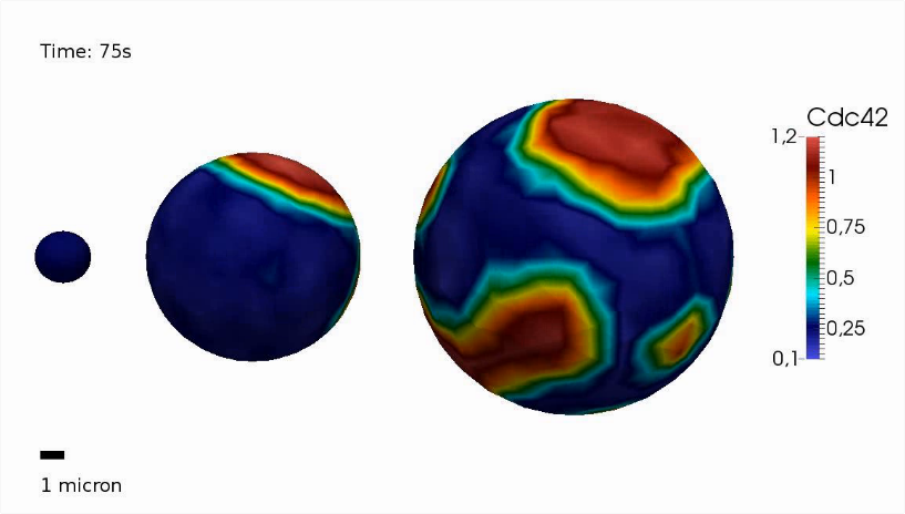
A partial differential equation (PDE) is an equation that contains partial derivatives in one or more variable(s). For instance, a PDE can be used to describe changes in time and space. Therefore, systems of PDEs can be considered as a natural extension of ODEs (ordinary differential equations). PDEs can be applied to a wide range of biological processes such as spatial signal transduction and cell-cell communication, mechanical forces in plant or fungal cell walls as well as membrane bending and stretching. While linear PDEs can often be invesigated analytically, solutions to non-linear PDE systems are usually obtained numerically by using the finite element method (FEM). -
Agent-based modeling
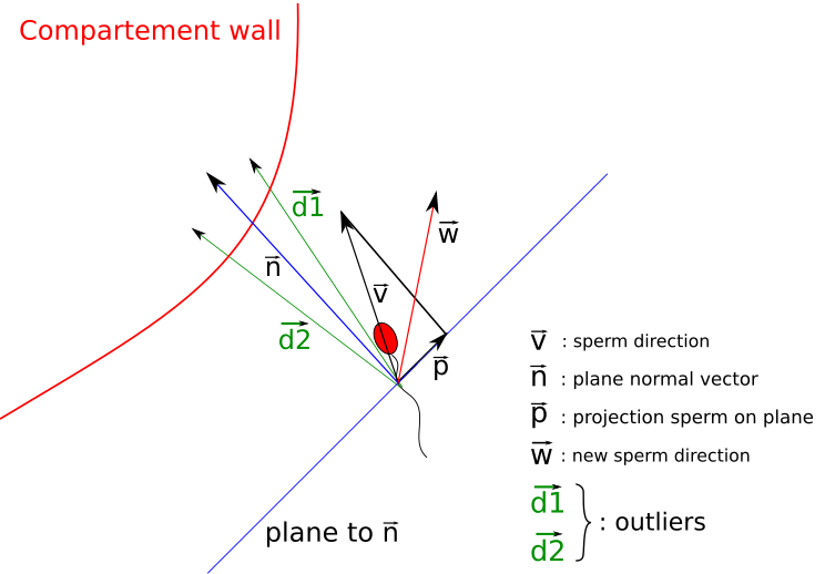
In agent-based modeling (ABM), a system is described as a collection of decision-making entities (agents) and a set of rules, which defines the agents' behaviour. The set of rules determines how agents interact which each other and/or their environment. Often, ABMs contain random elements, e.g. probabilistic decision making and initial agent placement. ABM provides a natural description of a biological system and is able to capture emergent (often unpredictable) behaviour. We use ABMs among others to model lipid metabolism, DNA repair or sperm migration. -
Boolean models
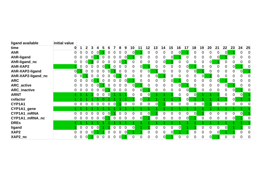
Boolean models are especially useful when rates and concentrations of a given system are unknown, as this type of model does not require kinetic parameters. It instead describes the system in a qualitative way. A Boolean network is defined as a set of nodes, which are influenced by other nodes in the network. Each node is defined by a Boolean variable, which can only take two values, TRUE and FALSE. To influence one another, nodes need transition functions, which dictate their behavior. In a biological system, the values TRUE and FALSE mostly represent the ON and OFF behavior of a biological component. Each node in a Boolean network represents such a biological component, for example a gene or a protein. The ON and OFF behavior signifies an activity, so ON means a protein or a gene is active, while OFF means it is inactive. In our group, we use Boolean models to represent large signaling networks. -

Stochastic models
Where molecule numbers are too small to be amenable to differential equation techniques, other modeling types have to be applied. This is the case in particular in protein translation, where both the number of mRNA transcripts and the number of produced protein molecules on biological time scales may be on the order of 1...10 for many genes. To avoid discretization errors, we treat every ribosome, mRNA transcript, tRNA molecule and protein individually and determine the reaction rates (initiation, elongation, termination) by means of random experiments. These models can accommodate time-dependent transcriptomes, energy dependence and tRNA numbers. -
Constraint-based modeling
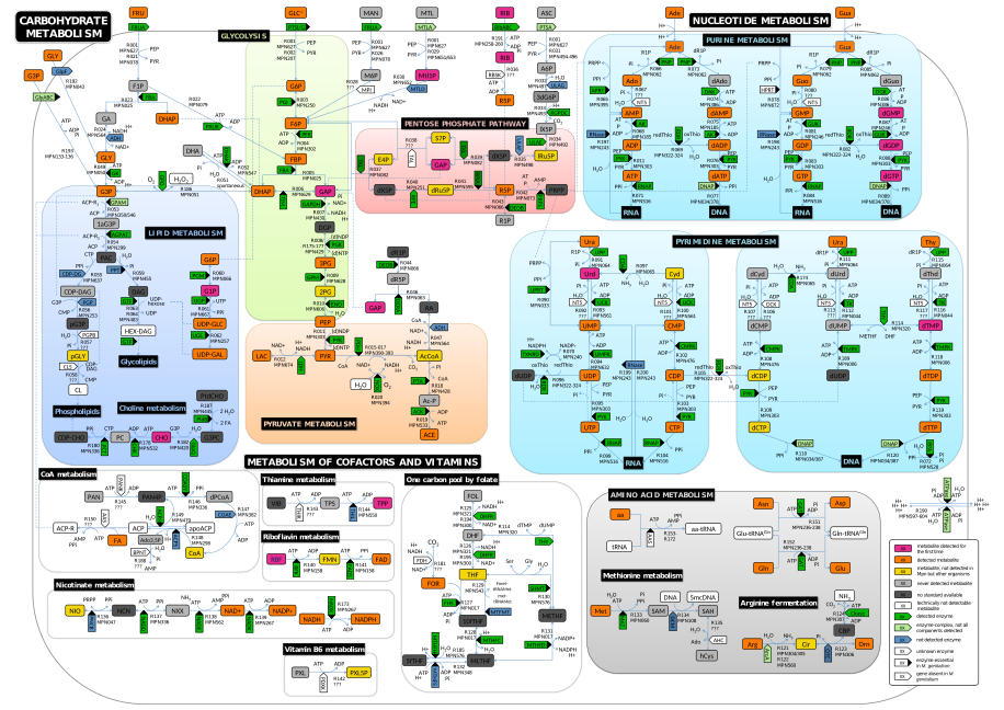
Constraint-based modeling is a static modeling approach applicable for large-scale metabolic networks. A constraint-based reconstruction is a union of (i) a stoichiometrically balanced metabolic model, (ii) a set of constraints for metabolic fluxes, and possibly (iii) a list of genes responsible for the catalysis of reactions included in the model. Detailed knowledge on species quantities, reaction mechanisms and the respective kinetic parameters (which are usually unknown) is not required. The genes - if known - are connected with the reactions by logical expressions. The constraints commonly limit available nutrients by setting maximum values for the source or the uptake reactions of sparse or known growth limiting nutrients. In addition, constraints can be used to define essential functions of the modeled networks, such as detoxification from metabolic by-products or the turnover of cellular entities such as mRNAs or proteins. Constraint-based models are commonly analyzed using flux balance analysis (FBA) or metabolic control analysis (MCA). Image from Yus et al., Science (2009). -
Reaction-contingency based modeling
Reaction-contingency based modeling is an approach to formalise molecular biology. It recognizes that we often have limited information of the exact nature of biochemical reactions. This is reflected by a separation between different possible events, “reactions”, and constraints on these events “contingencies”. The reactions capture the variables in the system by defining which state transitions may occur (e.g. protein-protein interactions, covalent modifications). The contingencies capture the causalities between these state transitions, e.g. that a kinase must bind a co-activator before phosphorylating a target. By defining both reactions and contingencies in terms of (combinations of) decontextualized, site-specific elemental states, the resolution of the model can be fully adapted to the underlying empirical data. In addition, the bipartite (reactions & contingencies) formalism makes the network definition scalable and composable, making it possible to accurately represent the state of the knowledge even for large networks. We have implemented this in the rxncon language, which is especially suited for formalising signal transduction. However, with the increasing awareness of metabolic regulation, it may also find its way into metabolic modeling.
- 1
DATA ANALYSIS
-
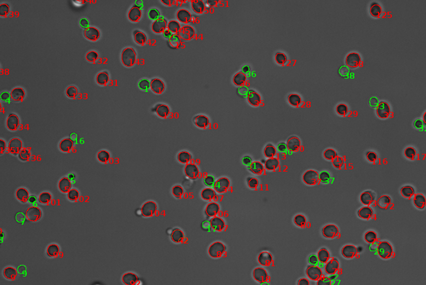
Image analysis
Image analysis involves the extraction of significant data from digital images. It requires processing techniques, by which data can be acquired and analyzed by a computer. Commonly used methods are for instance noise reduction, edge detection, and object recognition. Today, image analysis enables us to, among others, segment digital images and track particles. We use it to investigate cell morphologies and cellular processes. -
Analysis of periodic behaviour
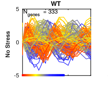
Periodic behavior is observed in many biological processes: Metabolite concentrations within cells can oscillate, the expression of genes is triggered in waves during the progression through the cell cycle, signaling pathways can show periodic activation. With systems theoretical approaches such as for example bifurcation analysis, we can identify the underlying reasons for this behavior, for example the effect of negative feedback loops. If the mechanistic structure of the system is unknown, we can also analyze oscillations only on the data level. For this we can use decomposition methods such as principal component analysis or Fourier transformations to identify different oscillatory patterns that might also be overlayed. We apply these techniques to the analysis of periodic gene expression in the yeast cell cycle or the measurement of the yeast cell wall rigidity and others. -
Machine learning
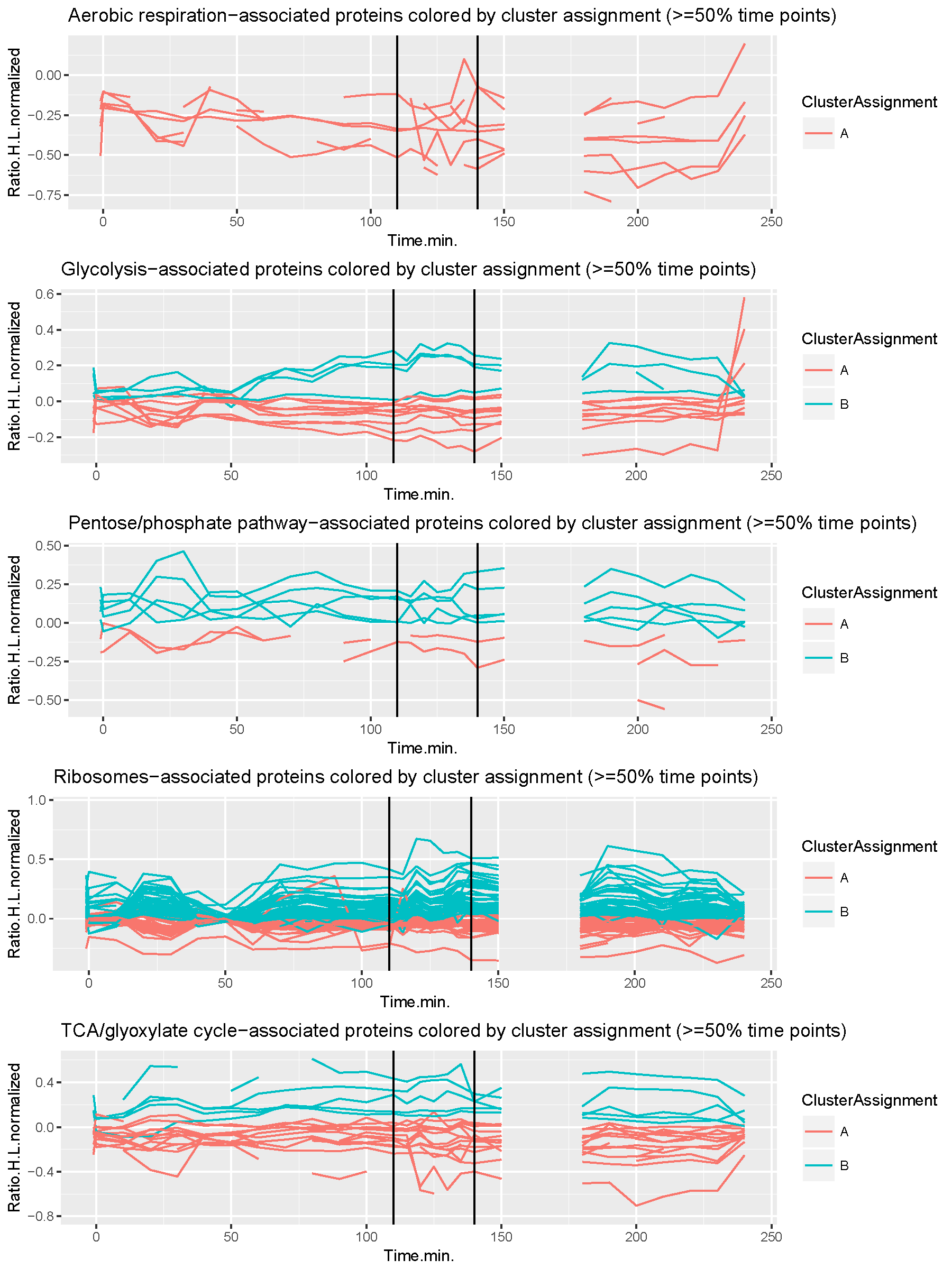
Machine learning is a complex tool at your disposal whenever it is necessary to find a common ground between entities (observations) in a dataset. Classification is a type of supervised learning, i.e. when some entities are already labelled towards a specific outcome. A classical example in computational biology are patients with a disease diagnosis and healthy individuals. Here, the challenge is to classify new, undiagnosed individuals (unlabeled observations) into one of the categories (healthy, disease) based on the same diagnostic data. This is solved by training a classifier which is an algorithm that finds patterns that are disease- and health-specific. The pattern found in an undiagnosed person (unlabelled entity) is then compared to the health- and disease-specific patterns. The higher similarity then decides which label is assigned to the undiagnosed person. There are multiple types of classifiers such as a Multilayer-Perceptron, Support-Vector-Machine, and Random-Forest to name a few. Clustering is another method and a type of unsupervised learning, hence there is no training data with representatives for each of the groups. In this scenario, the challenge is to find groups of entities (clusters) that are more similar to each other than to entities that belong to other clusters. This is a difficult problem when the number of clusters is not known prior to the clustering process. Hierarchical clustering elegently solves this problem by grouping all entities based on a decision-tree where the root are all entities together and the leaves are all entities individually. A depth cut-off then defines the resulting number of clusters and the cluster-assignments to each entity. Other clustering methods are K-means, Spectral-Clustering, Transitivity-Clustering, and many more. At the core of the clustering process is the similarity measure which is problem-specific and dependent on the experimental setup that produced the data. Time-series data, for example, require to identify similarities over the entire time-span of a measurement. Once clusters have been found, the next step is to extract the attribute(s) based on which the entities have been clustered together. This is called "feature extraction" which allows follow-up experiments to verify or falsify an underlying functional relationship of the observed statistical correlation. We have applied a clustering approach to time-series proteomics data of yeast cell over the cell cycle as shown here.
- 1
EXPERIMENTAL METHODS
-
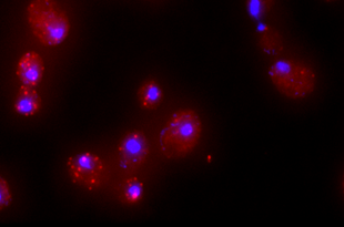
RNA FISH
RNA-FISH (fluorescence in situ hybridization) is the method of choice to quantify single mRNAs in fixed cells. Therefore, a set of approximately 48 single-labeled DNA probes complementary to the target genes are designed. After hybridization, mRNAs can be detected as single fluorescent spot using fluorescence microscopy and subsequently quantified. Using fluorescent cell cycle markers we are able to quantify mRNAs during specific cell cycle without any perturbation.
-
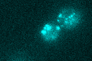
mRNA tracking (MS2)
We investigate the spatio-temporal dynamics of single mRNA molecules in living yeast cells using the MS2-system. This method exploits the high affinity of the viral coat protein of the bacteriophage MS2 - which we tag with fluorescent proteins - to certain stem-loop nucleotide sequences. In our lab, we genetically integrate these sequences into mRNAs of interest. The transcripts of the tagged gene become visible as the fluorescently tagged coat proteins accumulate on the stem-loop sequence. Importantly, all parts of this system are genetically encoded and no exogenous labels need to be added for imaging. We further develop this technique by improving fluorescent tags.
-
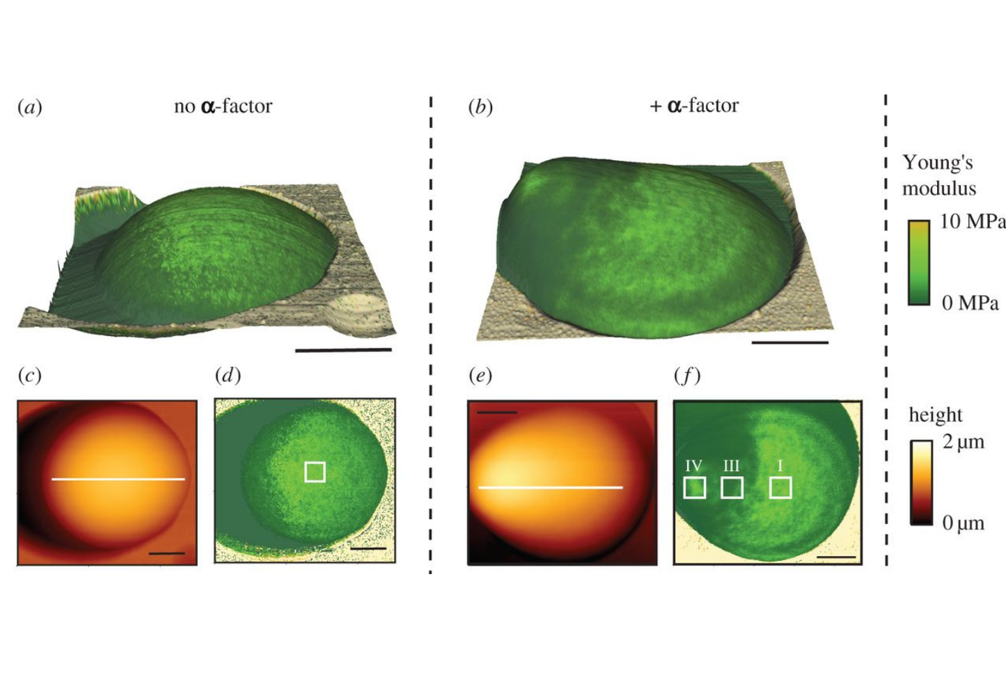
Cell wall mechanics and AFM
Atomic force spectroscopy (AFM) is a versatile tool to investigate surfaces with nanoscale precision. The method utilizes the deflection of a cantilever in response to tip surface interactions, thereby providing informations such as height or elasticity on a given position. Repeated measurements while scanning over defined areas can even provide maps of the parameter of interest. Using AFM we are able to determine the spatial distribution of mechanical cell wall properties during morphogenesis. (Image modified from Goldenbogen et al., Open Biol (2016), CC BY 4.0 license.)
-
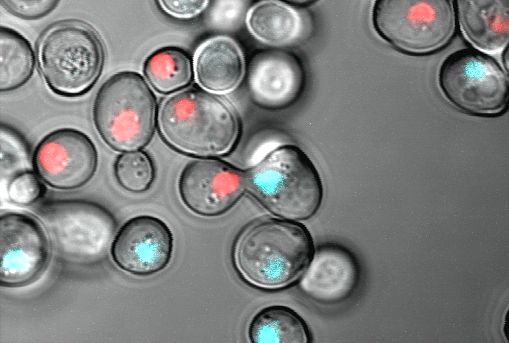
Fluorescence microscopy
With fluorescence microscopy, we visualize soluble proteins, organelles and structures like the nucleus, or the border between mother and daughter cell. Prerequisite for fluorescence microscopy is the existence of a fluorophore. We use often the green fluorescent protein or its derivatives to make proteins visible. In the image shown here, histones in the two yeast mating types are tagged with different fluorescent proteins a blue and a red fluorescent protein. The tagging with a fluorescent protein allows microscopy of living cells also for a time period.
-
FACS
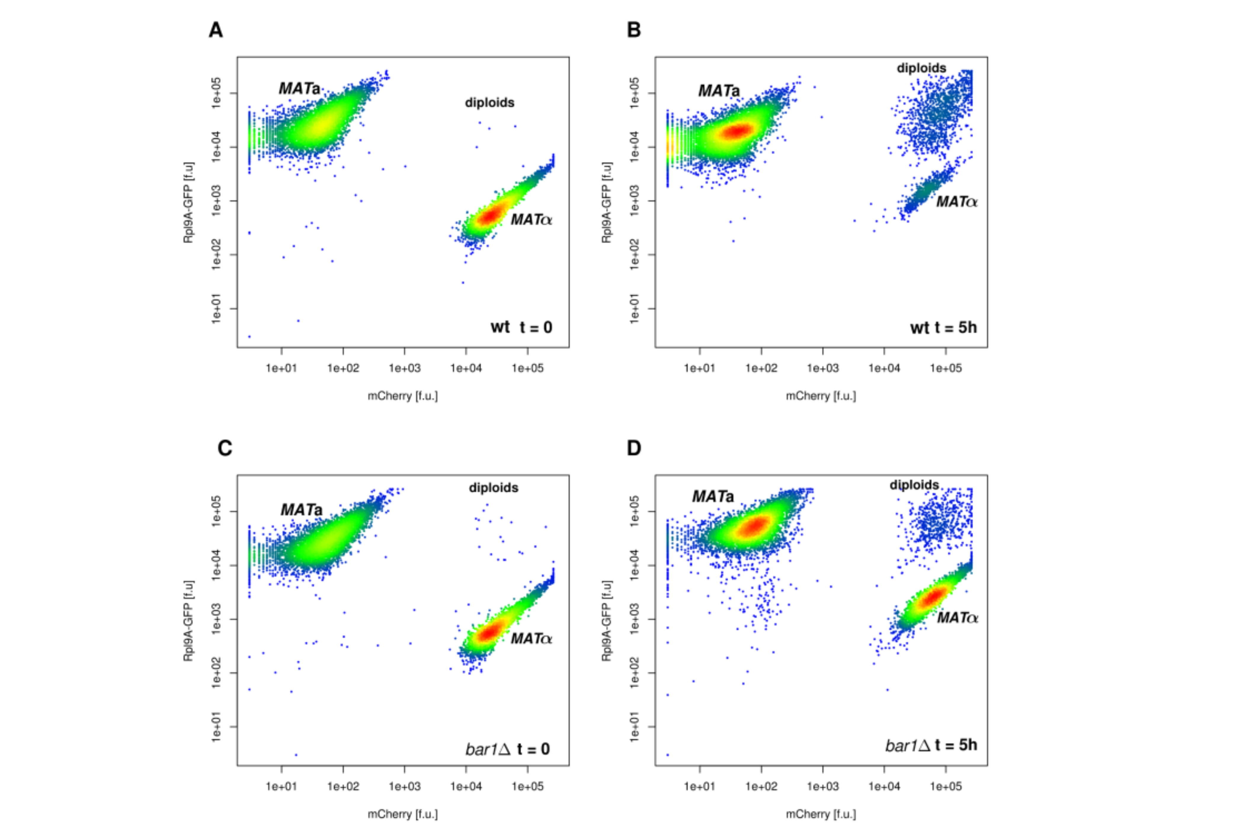
In FACS (Fluorescence Activated Cell Sorting) cells can be measured for size and several fluorescence channels simultaneously and can be sorted for a chosen feature. The cells flow past a laser beam, which excites the fluorophores and a detector measures the fluorescence and the scattered light. During the meassurement, cells can be sorted (e.g. for high or low fluorescence or size exclusion). Since FACS can be performed with living cells, the sorted cells can be grown in culture after the sorting.
-
Molecular biology
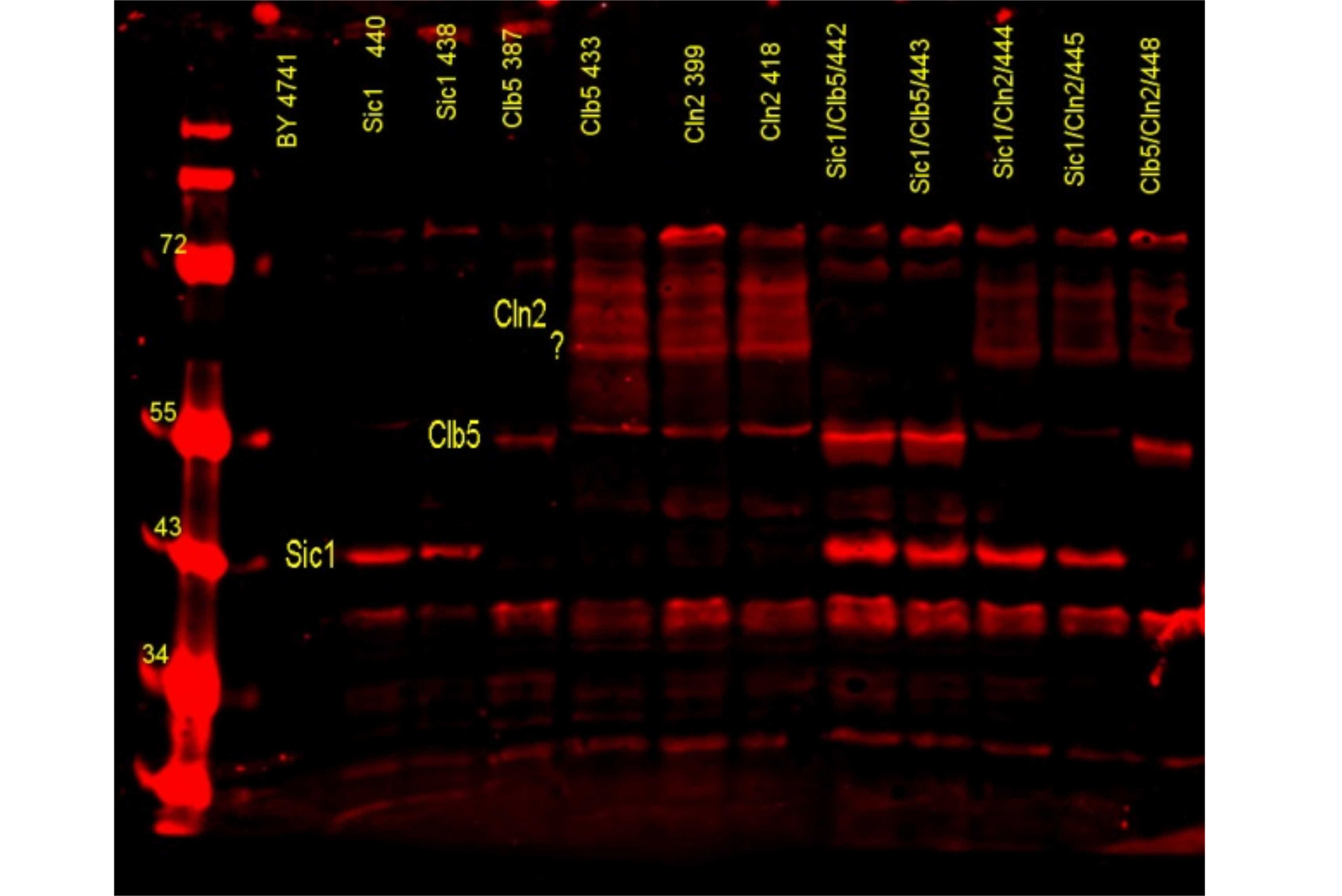
In our laboratory we make use of different techniques of molecular biology to alter and analyze the microorganism we wish to study. The general techniques include manupulation of DNA by PCR, Southern blot, ligation, digestion and recombination, analysis of RNA by Northern blot and Fluorescence in situ hibridization (FISH) and the detection and quantification of proteins by Western blot.
-

Synchronization
Synchronization of Saccharomyces cerevisiae can be achieved in different ways. First, block-and-release methods, where cells are synchronized in a specific cell cycle phase and released afterwards, can be used. Most prominent is the synchronization in G1 phase with alpha factor. Second, we use elutriation. For this synchronization method, cells are loaded in a specific centrifugation chamber. Using a buffer flow in the opposite direction of centrifugal force cells can be sorted depending on their size (surface/volume ratio). By increasing the flow we can washout and then harvest the smallest, new born G1 cells.
-
Cell size analysis
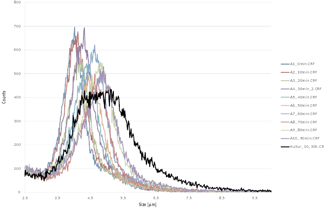
For rapid detection of cell number and size we use the CASY cell counting technology. Living cells, having an intact membrane are electric insulators. During measurement cells are passing through a pore and are exposed to an electric field. Being electric isolators cells increase the electric resistance in the pore, depending on the cell size. Dead cells are measured with the nucleus size. With help of the CASY Counter we are able to measure (i) cell number, (ii) cell size distribution.
- 1

